Here is a video I created describing how to use the scenario feature in open office calc.
Friday, November 28, 2008
Tuesday, November 25, 2008
Split Data in a Cell
Have you ever made a list of names in a spreadsheet and put the first and last name in one cell? Later on, you decide you want the first and last names to be in separate cells. Here is a video I created and posted on You Tube. Hope you enjoy.
For information on:
LEFT()
RIGHT()
LEN()
FIND()
you can see examples and explanations on my blog. Just look on the right hand side for the category the functions are in. They are grouped like they are in Calc.
For information on:
LEFT()
RIGHT()
LEN()
FIND()
you can see examples and explanations on my blog. Just look on the right hand side for the category the functions are in. They are grouped like they are in Calc.
Labels:
Video
Monday, November 24, 2008
FORECAST()
Extrapolates future values based on existing x and y values.
Syntax
FORECAST(Value; DataY; DataX)
Value is the x value, for which the y value on the linear regression is to be returned.
DataY is the array or range of known y's.
DataX is the array or range of known x's.
Cell D2 contains Value.
Cell E2 contains the formula =FORECAST(D2;$B$2:$B$40;$A$2:$A$40)
Cells E3:E12 contains formulas similar to the formula in E2.
Below is a screen shot of my spreadsheet.
Note: Not all of the x- and y-values are shown in the screen shot.
Labels:
Statistical Function
Saturday, November 22, 2008
Adding Just Odd Rows or Just Even Rows
Here is a neat little trick to add just the odd rows or just the even rows in a range.
Functions used in the formula.
SUM()
IF()
MOD()
ROW()
You can find an explanation of each of the above functions on my blog.
Adding just the odd rows.
C1 contains the formula
{=SUM(IF(MOD(ROW(A1:A10);2)=1;A1:A10;0))}
Notice the braces around the formula. You must enter it as an array formula (Ctrl>Shift>Enter)
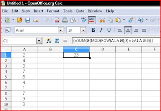
Adding just the even rows.
C1 contains the formula
{=SUM(IF(MOD(ROW(A1:A10);2)=0;A1:A10;0))}
Notice the braces around the formula. You must enter it as an array formula (Ctrl>Shift>Enter)
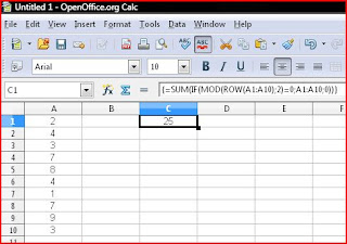
Notice the difference in the two formulas above. I have the differences highlighted in red.
We use a 1 in the formula to sum just the odd rows because whenever you divide an odd number by two you will get a remainder of one.
We use a 0 in the formula to sum just the even rows because whenever you divide an even number by two you will get a remainder of zero.
Functions used in the formula.
SUM()
IF()
MOD()
ROW()
You can find an explanation of each of the above functions on my blog.
Adding just the odd rows.
C1 contains the formula
{=SUM(IF(MOD(ROW(A1:A10);2)=1;A1:A10;0))}
Notice the braces around the formula. You must enter it as an array formula (Ctrl>Shift>Enter)

Adding just the even rows.
C1 contains the formula
{=SUM(IF(MOD(ROW(A1:A10);2)=0;A1:A10;0))}
Notice the braces around the formula. You must enter it as an array formula (Ctrl>Shift>Enter)

Notice the difference in the two formulas above. I have the differences highlighted in red.
We use a 1 in the formula to sum just the odd rows because whenever you divide an odd number by two you will get a remainder of one.
We use a 0 in the formula to sum just the even rows because whenever you divide an even number by two you will get a remainder of zero.
Labels:
Formulas
MOD()
MOD() - This function returns the remainder when one integer is divided by another.
Syntax:
MOD(Dividend;Divisor)
Example:
=MOD(25;4) returns 1
=MOD(38;9) returns 2
Syntax:
MOD(Dividend;Divisor)
Example:
=MOD(25;4) returns 1
=MOD(38;9) returns 2
Labels:
Mathematical Function
ROW()
ROW() - If a single cell is selected, this function returns the row number of a cell reference. If a range is selected, it returns the corresponding row numbers in a one-column array.
Note: If a cell range is selected, the formula must be entered as an array formula (Ctrl>Shift>Enter). If a range is selected and the ROW function is not entered as an array formula, only the the first range cell will be returned.
Example 1: The first example will return the row number a single cell reference.
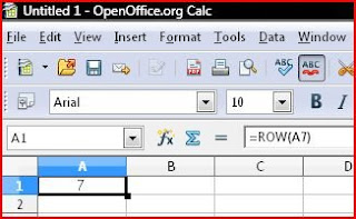
Cell A1 contains the formula =ROW(A7) which returns a value of 7.
Screen shot
Example 2: The second example will return the row numbers of a one-column array.
Cell A1 contains the formula {=ROW(B1:D5)} See screen shot below for results.
Notice the formula in the second example has braces around it. This is because the the function was entered as an array formula.
Screen shot

Note: If a cell range is selected, the formula must be entered as an array formula (Ctrl>Shift>Enter). If a range is selected and the ROW function is not entered as an array formula, only the the first range cell will be returned.
Example 1: The first example will return the row number a single cell reference.
Cell A1 contains the formula =ROW(A7) which returns a value of 7.
Screen shot

Example 2: The second example will return the row numbers of a one-column array.
Cell A1 contains the formula {=ROW(B1:D5)} See screen shot below for results.
Notice the formula in the second example has braces around it. This is because the the function was entered as an array formula.
Screen shot

Labels:
Spreadsheet Function
Friday, November 21, 2008
Format Paintbrush
The format paintbrush is a nice little tool that allows you to apply the attributes of currently selected cell to another cell or cells.
Select the cell whose attributes you want to copy.

Select the Format Paintbrush icon.
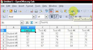
There will be a paint bucket next to the cursor. Select the cell or cells you want to apply the changes too. I did C1 to F1.

- Select the cell whose attributes you want to apply to another cell or cells.
- Click the Format Paintbrush icon on the toolbar.
- There will be a paint bucket next to the cursor. Select the cell or cells you would like to apply the changes too.
Select the cell whose attributes you want to copy.

Select the Format Paintbrush icon.

There will be a paint bucket next to the cursor. Select the cell or cells you want to apply the changes too. I did C1 to F1.

Labels:
Spreadsheet Features
Monday, November 3, 2008
Windows 7
Well microsoft is coming out with its new operating system. It is called Windows 7. Supposedly, they are shooting for simplicity. I was one of the unfortunate ones to get stuck with Vista. Microsoft knows it sucks. So what now. I have to dish out a couple of hundred bucks to get Windows 7. Why doesn't microsoft allow Vista users to have a free upgrade to Windows 7? I have never used an operating system as annoying as Vista. For the last time, I want to allow this. That gets so annoying. Microsoft's problem is they are trying to control what the user is doing. Let the people decide for themselves. So, come on microsoft, gives us unfortunate Vista users a break and let us have Windows 7 for free. After all, you are the ones that dumped this garbage on us.
Labels:
Software
HLOOKUP()
HLOOKUP() - This function searches across the top row in an array and returns a value in the same column in a specified row.
Syntax:
SearchCriteria - What you are wanting to match.
Array - The array you want to search through.
Index - Row number in the array from witch the matching value will be returned.
Sorted - If TRUE, HLOOKUP will look for an approximate match. If FALSE, HLOOKUP will look for an exact match.
Example:

I wanted to find the number of Highlander Hybrid's sold during the month of August. Below is the formula I have in cell "B22".
=HLOOKUP(I1;A1:M19;10;0)
"I1" represents the month I am looking for. I could have typed "August" instead of the cell address.
A1:M19 is the range I am looking through.
10 the row the Highlander Hybrid is in.
O which is the same as false means I want an exact match.
Syntax:
SearchCriteria - What you are wanting to match.
Array - The array you want to search through.
Index - Row number in the array from witch the matching value will be returned.
Sorted - If TRUE, HLOOKUP will look for an approximate match. If FALSE, HLOOKUP will look for an exact match.
Example:

I wanted to find the number of Highlander Hybrid's sold during the month of August. Below is the formula I have in cell "B22".
=HLOOKUP(I1;A1:M19;10;0)
"I1" represents the month I am looking for. I could have typed "August" instead of the cell address.
A1:M19 is the range I am looking through.
10 the row the Highlander Hybrid is in.
O which is the same as false means I want an exact match.
Labels:
Spreadsheet Function
Subscribe to:
Comments (Atom)
